High Frequency Trading
Feature Resampling
Tick data feeds are often aggregated into candlestick bars. Classical candlesticks are sampled with respect to time, but this choice is fairly arbitrary — for one, we know that markets do not trade at a uniform speed (Kyle & Obizhaeva, de Prado). For instance, market open and closing hours tend to be more liquid. Time bars oversample information during periods of low activity, and vice versa. Consequently, time sampling often exhibit poor statistical properties.
Sampling as a function of other variables, such as number of transactions (Mandelbrot, 1963), allows us to achieve samples closer to i.i.d. Gaussian distributions, making them more amenable to statistical modeling and interpretation.
Typical information included in aggregated bars include t (start), open, high, low, close, volume, n (number of ticks), vwap, T (end).
Let \( t_n \) be the current timestamp, then time bars are sampled when \(t_n > T\), where \( T = t + \tau \), a fixed interval length. We shall explore some alternative sampling methods.
- Tick Bars Set a constant tick count \(c\). Roll the bar when: \( n > c \).
- Volume Bars / Dollar Bars Analogous to tick bars, but triggered when total volume or dollar value exceeds a threshold.
Let a trade be defined by its timestamp, price, size, and direction, then
and for some \( \delta \) threshold, the samples are taken when
- Signed Tick Bars:
- Signed Volume Bars:
- Signed Dollar Bars:
Probabilistic Bars
So far, the bars are somewhat static, but we would like to perform sampling with frequency proprotional to the arrival of information. This new paradigm of information sampling works on a dynamic frequency with respect to deviation from some expected thresholds;
Define:
- \( n_{\text{ticks}} \): target number of ticks per bar
- \( \lambda \in [0,1] \): decay factor
Let:
- Tick imbalance:
- Average tick imbalance:
with expected value (exponential online estimate):
Then roll when:
Some Results A small numerical test is proposed to observe if BTC trade ticks exhibit mean-reversionary effects to vwap levels. Volume is often considered to be a metric of informed traders with asymmetric information crossing the bid-ask spread. It is reasonable to suspect that prices with higher volumes act as anchors. We test this relation using a simple regression relationship between time-series bar samples:
The trials are repeated for (i) classical time bars, and (ii) probabilistic bars. Data archival, restoration, tick data replay and regression analysis are all performed using quantpylib's features and Binance websocket data. See tick data management tutorial here. Documentation is here for the hft module. The code for regression trials and subscribing to the custom bar feeds is presented.
Code for Feature Resampling and Regression
import pytz
import json
import asyncio
import matplotlib.pyplot as plt

from datetime import datetime
from dateutil.relativedelta import relativedelta

import quantpylib.hft.bars as bars
from quantpylib.hft.feed import Feed
from quantpylib.gateway.master import Gateway

show = False
exc = 'binance'
tickers = ['BTCUSDT']
stream_data = {
    'binance': tickers,
}

run = None
time = None
replayer = None

from quantpylib.hft.mocks import Replayer,Latencies

hours = 10
now = datetime.now(pytz.utc)
start = now - relativedelta(hours=hours)
start = start.strftime('%Y-%m-%d:%H')
end = now.strftime('%Y-%m-%d:%H')

LATENCY = 0
latencies={
    Latencies.REQ_PUBLIC:LATENCY,
    Latencies.REQ_PRIVATE:LATENCY,
    Latencies.ACK_PUBLIC:LATENCY,
    Latencies.ACK_PRIVATE:LATENCY,
    Latencies.FEED_PUBLIC:LATENCY,
    Latencies.FEED_PRIVATE:LATENCY,
}
replayer_configs = {
    "latencies":latencies,
}

gateway = Gateway(config_keys={"binance": {}})

async def handler(bar):
    print(bar)

async def play_data(replayer,oms,feed,ticker):
    trade_feed_id = await feed.add_trades_feed(
        exc='binance',
        ticker='BTCUSDT',
        buffer=100,
    )
    time_bars = await feed.add_sampling_bars_feed(
        exc='binance',
        ticker='BTCUSDT',
        handler=handler,
        buffer=10000,
        bar_cls=bars.TimeBars,
        granularity='m',
        granularity_multiplier=3,
    )

    probabilistic_bars = await feed.add_sampling_bars_feed(
        exc='binance',
        ticker='BTCUSDT',
        handler=handler,
        buffer=10000,
        bar_cls=bars.ProbabilisticSignedTickBars,
        n_ticks=1500,
    )
    return time_bars,probabilistic_bars

async def hft(replayer,oms,feed):
    bar_feeds = await asyncio.gather(*[
        play_data(replayer=replayer,oms=oms,feed=feed,ticker=ticker)
        for ticker in tickers
    ])
    await run()
    for _type,_bar_feed in zip(['time','probabilistic'],bar_feeds[0]):
        bar_feed = feed.get_feed(_bar_feed)
        bars = bar_feed.as_df()

        from quantpylib.simulator.models import GeneticRegression
        configs = {"df":bars}

        model = GeneticRegression(
            formula="div(forward_1(c),c) ~ div(minus(c,vwap),c)",
            df=bars
        )
        res = model.ols()
        model.plot()
        print(res.summary())

async def sim_prepare():
    trade_data = {exchange:{} for exchange in stream_data}

    for exchange,tickers in stream_data.items():
        trade_archives = [
            Feed.load_trade_archives(
                exc=exchange,
                ticker=ticker,
                start=start,
                end=end
            ) for ticker in tickers
        ]

        trade_data[exchange] = {
            ticker:trade_archive
            for ticker,trade_archive in zip(tickers,trade_archives)
        }

    global replayer, run, time
    replayer = Replayer(
        l2_data={},
        trade_data=trade_data,
        gateway=gateway,
        **replayer_configs
    )
    oms = replayer.get_oms()
    feed = replayer.get_feed()
    run = lambda : replayer.play()
    time = lambda : replayer.time()
    return oms, feed

async def main():
    await gateway.init_clients()
    oms,feed = await sim_prepare()
    await oms.init()
    await hft(replayer,oms,feed)
    await gateway.cleanup_clients()

if __name__ == '__main__':
    asyncio.run(main())
The sampled bars are retrieved as in bar_feed.as_df()
                t         o         h         l         c        v       n           vwap             T
0    1.747516e+12  103330.7  103376.4  103286.5  103286.5  102.308  1389.0  103340.333948  1.747516e+12
1    1.747516e+12  103286.6  103350.0  103248.8  103349.9   93.656  1317.0  103297.011811  1.747516e+12
2    1.747516e+12  103350.0  103458.6  103280.1  103280.1  280.711  2457.0  103403.270401  1.747516e+12
3    1.747516e+12  103280.1  103301.2  103262.4  103301.2   74.626  1001.0  103276.858821  1.747516e+12
4    1.747516e+12  103301.2  103390.2  103301.1  103356.7  105.848   884.0  103353.044096  1.747516e+12
..            ...       ...       ...       ...       ...      ...     ...            ...           ...
196  1.747551e+12  103417.6  103431.9  103350.4  103359.1  112.305  1143.0  103395.879483  1.747551e+12
197  1.747551e+12  103359.2  103382.8  103350.7  103350.8   57.124   942.0  103366.522973  1.747551e+12
198  1.747551e+12  103350.8  103353.8  103320.0  103353.7   82.479   838.0  103339.882634  1.747551e+12
199  1.747551e+12  103353.7  103386.8  103353.7  103370.6   61.202   714.0  103366.291206  1.747551e+12
200  1.747551e+12  103370.7  103429.4  103353.8  103414.4  144.935  1389.0  103390.268834  1.747552e+12
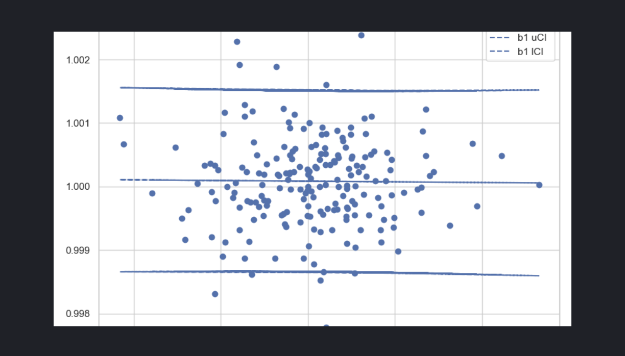
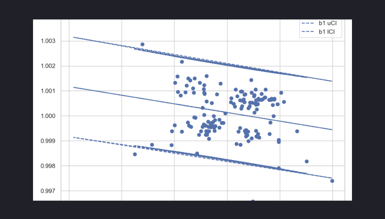
We obtained the following results for time-based sampling (not significant) and probabilisitic sampling (significant)
                            OLS Regression Results
==============================================================================
Dep. Variable:                     b0   R-squared:                       0.000
Model:                            OLS   Adj. R-squared:                 -0.005
Method:                 Least Squares   F-statistic:                   0.02410
Date:                Tue, 13 May 2025   Prob (F-statistic):              0.877
Time:                        21:34:09   Log-Likelihood:                 1170.6
No. Observations:                 201   AIC:                            -2337.
Df Residuals:                     199   BIC:                            -2331.
Df Model:                           1
Covariance Type:            nonrobust
==============================================================================
                 coef    std err          t      P>|t|      [0.025      0.975]
------------------------------------------------------------------------------
Intercept      1.0001   5.08e-05   1.97e+04      0.000       1.000       1.000
b1            -0.0209      0.135     -0.155      0.877      -0.286       0.244
==============================================================================
Omnibus:                       11.897   Durbin-Watson:                   1.867
Prob(Omnibus):                  0.003   Jarque-Bera (JB):               19.713
Skew:                           0.315   Prob(JB):                     5.24e-05
Kurtosis:                       4.399   Cond. No.                     2.65e+03
==============================================================================

XXXXXXXXXXXXXXXXXXXXXXXXXXXXXXXXXXXXXXXXXXXXXXXXXXXXXXXXXXXXXXXXXXXXXXXXXXXXXX

                            OLS Regression Results
==============================================================================
Dep. Variable:                     b0   R-squared:                       0.059
Model:                            OLS   Adj. R-squared:                  0.053
Method:                 Least Squares   F-statistic:                     9.050
Date:                Tue, 13 May 2025   Prob (F-statistic):            0.00310
Time:                        21:34:28   Log-Likelihood:                 809.41
No. Observations:                 146   AIC:                            -1615.
Df Residuals:                     144   BIC:                            -1609.
Df Model:                           1
Covariance Type:            nonrobust
==============================================================================
                 coef    std err          t      P>|t|      [0.025      0.975]
------------------------------------------------------------------------------
Intercept      1.0001   7.89e-05   1.27e+04      0.000       1.000       1.000
b1            -0.3461      0.115     -3.008      0.003      -0.573      -0.119
==============================================================================
Omnibus:                        3.589   Durbin-Watson:                   2.021
Prob(Omnibus):                  0.166   Jarque-Bera (JB):                3.380
Skew:                          -0.215   Prob(JB):                        0.184
Kurtosis:                       3.608   Cond. No.                     1.46e+03
==============================================================================
Clearly, the numerical experiments reveal some interesting dynamics between sampling behaviour and the presence of mean-reversion effects. Not as clearly, it is important to keep in mind these are time-varying effects, and most perhaps regime dependent.